About AMR and R package
R package to simplify the analysis and prediction of Antimicrobial Resistance (AMR) and to work with microbial and antimicrobial data and properties, by using evidence-based methods. Copyright by: https://msberends.github.io/AMR/index.html#copyright
Outine
- R packages installation
- Import CSV data
- Find frequency by variables
- Find resistance percentages
- Find resistance percentages by organism and number of isolates
- Calculate empiric susceptibility
- Calculate empiric susceptibility - Percentage
- Plotting results and compare susceptibility by antibiotics
- Yearly isolates summary - Bar chart
1. R packages installation
Open your R-Studio and install the following packages:
install.packages(c("dplyr", "ggplot2", "AMR", "cleaner"))
After successful installtion, Import the libraries:
library(dplyr)
library(ggplot2)
library(AMR)
library(cleaner)
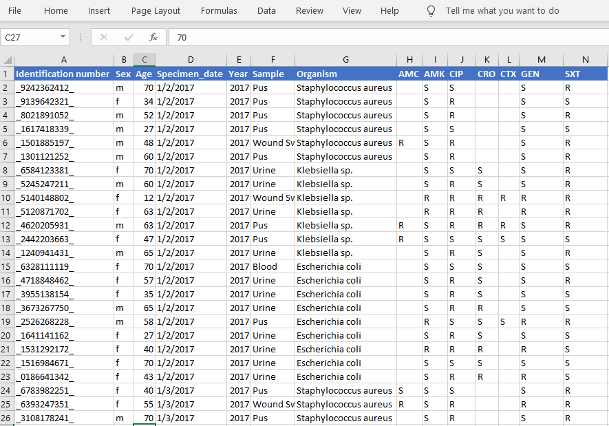
2. Import CSV data
# Import excel/csv data
data_sample <- read.csv("Your-file-location/amr-sample-data-r-analysis.csv")
head(data_sample) # AMK = Amikacin, AMC = Amoxicillin / Clavulanic Acid,  CIP = Ciprofloxacin,
                  # CTX = cefotaxime, SXT = Trimethoprim/Sulfamethoxazole, CRO = Ceftriaxone
Output:
3. Find frequency by variables
data_sample %>% freq(Sex)
data_sample %>% freq(Organism)
data_sample %>% freq(Sample)

Output-Sex:
Frequency table

Class:      character
Length:     23,411
Available:  23,411 (100.0%, NA: 0 = 0.0%)
Unique:     2

Shortest:   1
Longest:    1

     Item       Count    Percent    Cum. Count    Cum. Percent
---  ------  --------  ---------  ------------  --------------
1    f         13,568     57.96%        13,568          57.96%
2    m          9,843     42.04%        23,411         100.00%


Output-Organism:

Frequency table

Class:      character
Length:     23,411
Available:  23,411 (100.0%, NA: 0 = 0.0%)
Unique:     3

Shortest:   14
Longest:    21

     Item                        Count    Percent    Cum. Count    Cum. Percent
---  -----------------------  --------  ---------  ------------  --------------
1    Escherichia coli           11,887     50.78%        11,887          50.78%
2    Klebsiella sp.              7,709     32.93%        19,596          83.70%
3    Staphylococcus aureus       3,815     16.30%        23,411         100.00%

Output-Sample:

Frequency table

Class:      character
Length:     23,411
Available:  23,411 (100.0%, NA: 0 = 0.0%)
Unique:     6

Shortest:   3
Longest:    10

     Item             Count    Percent    Cum. Count    Cum. Percent
---  ------------  --------  ---------  ------------  --------------
1    Urine           12,814     54.73%        12,814          54.73%
2    Pus              5,753     24.57%        18,567          79.31%
3    Wound Swab       2,549     10.89%        21,116          90.20%
4    Blood            1,214      5.19%        22,330          95.38%
5    Sputum           1,079      4.61%        23,409          99.99%
6    Stool                2      0.01%        23,411         100.00%
4. Overview of different bug/drug combinations
# Number of isolates in different bug/drug combinations

data_sample %>%
  bug_drug_combinations() %>%
  head(100) # show 100 rows

Results:
         mo    ab   S   I  R   total
1     E. coli AMC  3163 0 8484 11647
2     E. coli AMK 10541 2 1215 11758
3     E. coli CIP  3148 0 8710 11858
4     E. coli CRO  3741 0 8118 11859
5     E. coli CTX   483 0 1575  2058
6     E. coli GEN  9301 0 2487 11788
7     E. coli SXT  5408 1 6438 11847
8  Klebsiella AMC  2261 0 5360  7621
9  Klebsiella AMK  4818 1 2843  7662
10 Klebsiella CIP  2777 6 4904  7687
11 Klebsiella CRO  2626 0 5054  7680
12 Klebsiella CTX  1358 0 3799  5157
13 Klebsiella GEN  4461 0 3182  7643
14 Klebsiella SXT  2984 0 4687  7671
15  S. aureus AMC  2208 0 1388  3596
16  S. aureus AMK  3476 0  291  3767
17  S. aureus CIP  1228 0 2573  3801
18  S. aureus CRO     6 0    2     8
19  S. aureus CTX     2 0    3     5
20  S. aureus GEN  3359 0  422  3781
21  S. aureus SXT  2523 0 1272  3795


# For `aminoglycosides()` using column 'GEN' (gentamicin)
data_sample %>%
  select(col_mo, aminoglycosides()) %>%
  bug_drug_combinations()

Result:

        mo   ab     S  I  R   total
1    E. coli AMK 10541 2 1215 11758
2    E. coli GEN  9301 0 2487 11788
3 Klebsiella AMK  4818 1 2843  7662
4 Klebsiella GEN  4461 0 3182  7643
5  S. aureus AMK  3476 0  291  3767
6  S. aureus GEN  3359 0  422  3781
5. Find resistance percentages
data_sample %>% resistance(AMC)

Output:

0.6662001
6. Find resistance percentages by organism and number of isolates
data_sample %>%
  group_by(Organism) %>%
  summarise(amoxiclav = resistance(AMC),
            #amoxiclav_isolates = n_rsi(AMC),
            gentamicin = resistance(GEN),
            #gentamicin_isolates = n_rsi(GEN),
            ciprofloxacin = resistance(CIP),
            #ciprofloxacin_isolates = n_rsi(CIP)
            )

Output:

  Organism              amoxiclav gentamicin ciprofloxacin
1 Escherichia coli          0.728      0.211         0.735
2 Klebsiella sp.            0.703      0.416         0.638
3 Staphylococcus aureus     0.386      0.112         0.677

-----------------------------------------------------------
# Total number of isolates responsible for the percentages by group (S, I or R)

data_sample %>%
  group_by(col_mo) %>%
  summarise(amoxiclav = resistance(AMC),
            #amoxiclav_isolates = n_rsi(AMC),
            gentamicin = resistance(GEN),
            #gentamicin_isolates = n_rsi(GEN),
            ciprofloxacin = resistance(CIP),
            #ciprofloxacin_isolates = n_rsi(CIP)
            total_isolates = n_rsi(SXT))

Output:
col_mo           amoxiclav gentamicin ciprofloxacin   total_isolates
1 B_ESCHR_COLI     0.728      0.211         0.735          11847
2 B_KLBSL          0.703      0.416         0.638           7671
3 B_STPHY_AURS     0.386      0.112         0.677           3795


-----------------------------------------------------------
# For the resistance within certain antibiotic classes, use a antibiotic class selector
such as penicillins(), which automatically will include the columns AMX and AMC of our data


data_sample %>%
  summarise(across(penicillins(), resistance, as_percent = TRUE)) %>%
  rename_with(set_ab_names, penicillins())

Output:
  amoxicillin_clavulanic_acid
1                       66.6%

-----------------------------------------------------------
7. Calculate empiric susceptibility: Get the proportion of multiple antibiotics, to calculate empiric susceptibility of combination therapies
data_sample %>%
  group_by(Organism) %>%
  summarise(amoxiclav = susceptibility(AMC),
            gentamicin = susceptibility(GEN),
            amoxiclav_genta = susceptibility(AMC, GEN))

Output:

  Organism              amoxiclav gentamicin amoxiclav_genta
1 Escherichia coli          0.272      0.789           0.804
2 Klebsiella sp.            0.297      0.584           0.592
3 Staphylococcus aureus     0.614      0.888           0.907
8. Calculate empiric susceptibility - Percentage
data_sample %>%
  group_by(Organism) %>%
  summarise(across(penicillins(), resistance, as_percent = TRUE))

Output:

  Organism              AMC
1 Escherichia coli      72.8%
2 Klebsiella sp.        70.3%
3 Staphylococcus aureus 38.6%
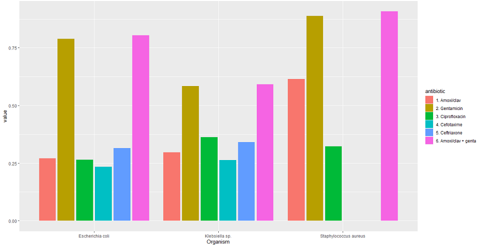
9. Plotting results and compare susceptibility by antibiotics
data_sample %>%
  group_by(Organism) %>%
  summarise("1. Amoxi/clav"    = susceptibility(AMC),
            "2. Gentamicin"    = susceptibility(GEN),
            "3. Ciprofloxacin" = susceptibility(CIP),
            "4. Cefotaxime"    = susceptibility(CTX),
            "5. Ceftriaxone"  = susceptibility(CRO),
            "6. Amoxi/clav + genta" = susceptibility(AMC, GEN)) %>%
  tidyr::pivot_longer(-Organism, names_to = "antibiotic") %>%
  ggplot(aes(x = Organism,
             y = value,
             fill = antibiotic)) +
  geom_col(position = "dodge2")

Output:
10. Stacked bars for SI and R
ggplot(data_sample) +
  geom_rsi(translate_ab = FALSE

Output: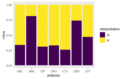
11. Resistance per genus and antibiotic
# group the data on `genus`
ggplot(data_sample %>% group_by(col_mo)) +
  geom_rsi(x = "col_mo") +

  facet_rsi(facet = "antibiotic") +
  # set colours to the R/SI interpretations (colour-blind friendly)
  scale_rsi_colours() +
  # show percentages on y axis
  scale_y_percent(breaks = 0:4 * 25) +
  # turn 90 degrees, to make it bars instead of columns
  coord_flip() +
  # add labels
  labs(title = "Resistance per genus and antibiotic")
  # and print genus in italic to follow our convention
  # (is now y axis because we turned the plot)
  theme(axis.text.y = element_text(face = "italic"))

Output: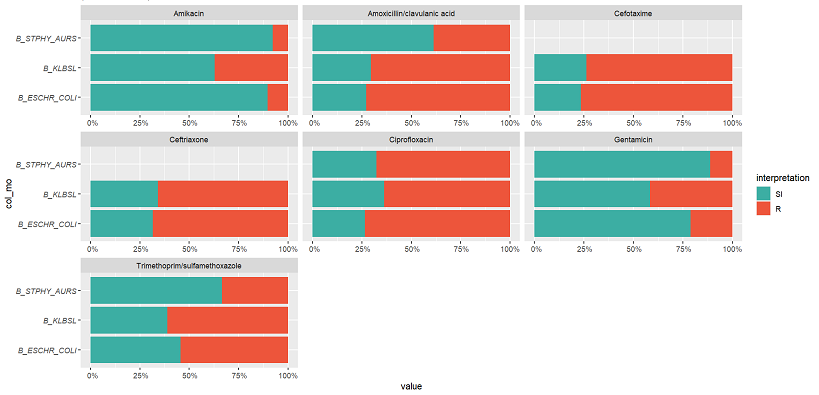
12. Yearly isolates summary - Bar chart
ggplot(data_sample) +
  geom_bar(aes(Year))

Output: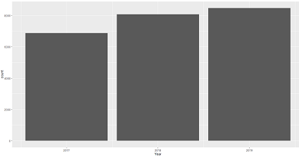
Source: https://msberends.github.io/AMR/articles/AMR.html